Modelling Survival in Old Age: Multinomial outcome

Said Shahtahmasebi, PhD

The Good Life Research Centre Trust, Christchurch, New Zealand.

Correspondence: email: radisolevoo@gmail.com

Key words: multinomial, statistical modelling, longevity

Received: 29/12/2019; revised 5/2/2020; Accepted: 25/2/2020

[citation: Shahtahmasebi, S. (2020). Modelling Survival in Old Age: Multinomial outcome. DHH, 7(1):http://www.journalofhealth.co.nz/?page_id=2057].

Introduction

An earlier paper investigated survival in old age as a dichotomy (alive or deceased) using data from the North Wales Elderly Project (NWEP) (Shahtahmasebi, 2019), for more details see (Shahtahmasebi & Berridge, 2010).

Although, the statistical modelling allowed control for multicollinearity and simplified the number of variable reported to be associated with survival, there still remains unaccounted confounding and sources of bias. For example, at the end of the project some had died, some were still alive and were living in the community, and some were alive but living in residential care. Therefore, the additional information about survivors is not used in the analysis of survival based on only two possible outcomes, i.e. lumping all survivors in the alive category ignores various degrees of dependency in old age. Furthermore, such a mix will lower the average duration or age of survival and thus underestimates the probability of survival.

Fortunately, in the NEWP the status of the sample members can be ascertained at each interval point to form a multinomial survival outcome, which makes it possible to increase complexity in the methodology.

In this paper I demonstrate insight gained by utilising the additional information in a more complex methodology.

Multinomial survival

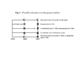
In the earlier paper (Shahtahmasebi, 2019), the probability of being a survivor (or deceased) after eight years for an elderly individual in the sample was investigated. This was done by combining together all survivors, regardless of their degree of frailty, as one category and all deceased, regardless of when they died during the project window, as another category. However, in old age, the ‘path’ to death could be viewed as a sequential process as shown in Figure 1. All individuals were alive and in the community at the start of the project. Over the subsequent years, some became dependent before death and some were still in the community. One outcome that could be used to measure dependency prior to death is entry into residential care. Therefore it is reasonable to distinguish between two types of survivor: survivors in the community and survivors in residential care. Such a distinction provides a more detailed, and potentially more insightful, response variable of survival in old age and makes more use of the data available. The outcome now has three possible events: survivor in the community, survivor in residential care and deceased. In this case, the binary logistic regression applied in the previous paper is no longer appropriate. This paper concentrates on the application of a more complex family of multinomial response models for ordered outcome processes.

Fig. 1 here

Statistical modelling

Multinomial response data can be modelled by specifying and fitting a general multinomial model to the data. This means that the response has three or more possible outcomes each of which has a non-zero probability of occurring (see Appendix).

Model Specification

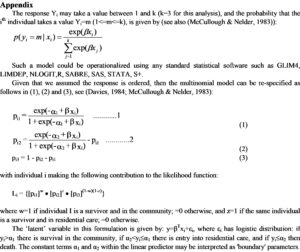
All the elderly respondents in the project were alive and in the community at the start of the project. Some elderly respondents entered residential care, and some died. As illustrated in Fig. 1 we can assume sequential ordinality in the three response categories (‘in the community’, ‘in care’ and ‘deceased’) leading to a special case of the multinomial response model. This is equivalent to assuming some latent variable which measures the degree of dependence or frailty (see Fig. 2); at high levels of this latent variable, individuals are expected to be in the community but when they cross over some threshold of dependence they would enter residential care. Lower levels of this variable are associated with death. In other words, we could regard the latent variable in two ways: first, as a dependency measure; second, as an indicator of the strength of independence of an individual. The lower the independence, the greater are the levels of dependency and the higher is the chance of death.

Individuals with identical observed characteristics may have different outcomes (e.g. one may be in the community, another in residential care) because of the unobserved variables and elements of chance in the factors involved. The model is operationalized in terms of the probabilities of outcomes to allow for these uncertainties (see Appendix, Shahtahmasebi & Berridge, 2010). However, the formal latent variable formulation permits us to quantify the effect of specific factors on the probability of different outcomes.

We proceed by assuming the probability of an individual falling in any of the response categories to be a logit function of the explanatory variables, see Appendix.

Figure 2 – Logistic function relating known outcomes to unknown latent variable.

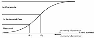
The formulation for the ordered multinomial model (see Appendix, also see Shahtahmasebi & Berridge, 2010) is demonstrated in Figure 2. The ‘latent’ variable in this formulation is given by the response y: if y_i>α₁ there is survival in the community, if α₂<y_i£α₁ there is entry into residential care, and if y_i£α₂ then death. Other ordinal specifications are possible (McCullough, 1980), but the approach adopted here has the advantage of needing only a single linear predictor (see also (Davies, 1984)).

At the time of the analysis it was not possible to use standard statistical packages to fit such a multinomial model to the data. Thus, in-house FORTRAN programs were developed to cope with routine algebra/matrix calculations involved with the likelihood estimation, likelihood ratio statistic (χ²) and associated p-values. However, nowadays such a model may be fitted to data routinely using statistical software packages, e.g. the freely available SABRE (Shahtahmasebi & Berridge, 2010).

Variable Selection

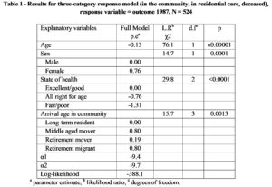
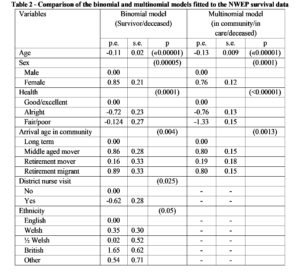
A forward iterative variable selection method was used in which variables were entered in the model one at a time and their effects, based on the c² test statistic, were noted. The variable with the largest c² and smallest p-value was selected for inclusion in the model first and the model-building process then continued until no further variables remained significant at the 5% level. The results were then checked for the possibility of alternative models e.g. where the difference between two effects may be too small to be distinguishable or where practical significance took priority over statistical significance. There were no causes for concern. The list of variables and model fitting results are shown in table 1.

Table 1 – Results for three-category response model (in the community, in residential care, deceased), response variable = outcome 1987, N = 524

 

Interpretation

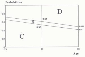
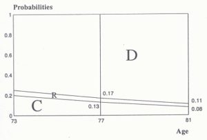
The interpretation can be assisted by the probability curve in Fig. 2. The probability of a latent variable value between α₁ and α₂ specifies the probability of an individual being in residential care, below α₂ indicates the probability of death for an individual with the same age; and above α₂ indicates the probability of remaining in the community. Table 1 only provides an indication of the direction of the effect, e.g. a negative effect implies a lower probability of survival and a positive effect implies a higher probability of survival. The rationale behind Fig. 2 was used to construct Figures 3-5. These figures show plots of cumulative probabilities for different effects against age with other variables set to their reference category values as appropriate. The probability of going into care is represented by the area (R) between the areas representing probability of survival in the community (C) and probability of death (D). The results from Table 1 were substituted into equations (1‑3, see Appendix) to estimate these probabilities. Including interactions in the model would have provided a more flexible specification but this was not possible due to the limited size of these data.

As would be expected, Table 1 indicates that the older the respondents, the less likelihood of survival in the community and that female respondents are more likely to survive in the community. It can be seen from Figure 3 that the probability of survival in the community after eight years (1979‑87, from Table 1) for those who are a male, in good/excellent health, and a long-term resident decreases from 0.48 at age 73, to 0.35 at 77, and to 0.24 at age 81 (remember that the youngest member of the sample was 65 in 1979).

Figure 3 – Diagrammatical representation of the multinomial response probability distribution given observed age.

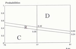
However, while the probability of death is monotone increasing (i.e. from 1.0- 0.55=0.45 at age 73, to 1.0‑0.42=0.58 at 77, and to 1.0‑0.30=0.70 at 81), the probability of being in care appears to be fairly constant (i.e. from 0.55‑0.48=0.07 at age 73, to 0.42‑0.35=0.07 at age 77, and to 0.30- 0.24=0.06 at 81).

Because of the importance of age, it was used as a ‘base’ when considering other effects. The variable sex is significant. To see how elderly males compare with elderly females, the results from Table 1 were substituted into formulae (1) and (2) in Appendix controlling for age. The resulting probabilities were used to construct the probability diagrams shown in Figures 2.4 (a) and (b). By comparing Figure 2.4(a) with Figure 2.4(b), the differences between men and women can be explored. For instance, at the age of 73, women are about 38% (0.66/0.48=1.38) more likely to remain in the community than men. Women appear to be more likely to survive longer in the community and hence may enter into care at an older age. Using such a decomposition we proceed with the interpretation of the remaining effects.

Figure 4.

(a) multinomial probability of survival of a female for observed age, from Table 1.

(b) multinomial probability of survival of a male individual given observed age, from Table 1.

There is strong evidence to suggest that poor health is related to non-survival in the community. It can be seen that the likelihood of non-survival in the community increases as (self-assessed) state of health declines (Table 1). This is reflected in its negative parameter estimates (e.g. -0.76 for ‘all right for age’ and -1.31 for ‘fair/poor’).

Self-assessed state of health appears to influence the outcome probability in the sense that poorer health appears to accelerate leaving the community. This is again illustrated in Figures 5 (a) and (b). It can be seen that, over the period 1979‑87 (Table 1) those 73 year olds (who were 65 in 1979) who in 1979 assessed their health to be ‘fair/poor’ are 2.4 times less likely to remain in the community and 1.7 times more likely to have died by 1987 than other 73 year olds who claimed to be in a ‘good’ state of health. Elderly individuals enter into residential care for several reasons, e.g. loneliness (Booth & Bilson, 1988; Dykstra, van Tilburg, & Gierveld, 2005). Some studies suggest residential care causes loneliness whilst Dykstra and colleagues (Dykstra et al., 2005) suggested that entering residential care does not reduce loneliness. Deterioration of health in old age prompts more contacts, care and visits from close relatives, friends and neighbours (Wenger, 1989). This may, at least in part, explain why those in poor health have a lower probability of entry into residential care. Therefore, as shown in Figure 5(a), elderly individuals with a low probability of remaining in the community, possibly due to poor health, will have a high probability of dying, thus a low probability of entry into care. On the other hand, Figure 5(b) suggests that those elderly in good health appear to have a higher probability of remaining in the community and a lower probability of death and a slightly higher probability of entry into residential care.

Figure 5.

(a) multinomial probability of survival for individuals in ‘fair/poor’ health for observed age, from Table 1.

(b) multinomial probability of survival for individuals in ‘good’ health for observed age, from table 1.

The variable ‘arrival age in community’ appears to be positively linked with survival. There is strong evidence to support its inclusion in the model for the period 1979‑87 (p=0.0013, Table 1). This suggests a long-term effect. Middle aged movers and retirement migrants (those who have moved more than 25 miles after the age of 60) have a greater chance of survival than retirement movers (those who move short distances after the age of 60 – this group tends mainly to be locals). There is a degree of association between this variable, social class and network type (Shahtahmasebi & Wenger, 1989). The duration of staying in the community can reflect availability of kin; those who arrived in the community before or during child-rearing age are more likely to have a local kin network than those who arrived in middle or old age. Moreover, movement by those in the lower social class appears to take place mainly within the community. In this model, the variable ‘arrival age in community’, therefore, appears to control for the effects of both social class and network type.

Summary

To see how the multinomial model performs in comparison with the binomial logistic model reported earlier (Shahtahmasebi, 2019), the results from the two models are reproduced in Table 2. Notice that for this table we have chosen to present parameter estimates (p.e.’s) along with their standard errors (s.e.’s) and associated p-values. This is the conventional way of presenting the results of fitting models but our main reason here is a comparison of the two models. Here we are not exploring how variables fit in a model but how models compare with each other. Although, ideally, both model should have had the same variables included to be able to compare p.e.’s and s.e.’s. Nevertheless, we are still able to compare the two models and use p.e.’s and s.e.’s as a guide.

In general, the p.e.’s are very similar but those of the multinomial model have much smaller s.e.’s. This may be evidence of a more powerful model because fuller use is made of the response data, but this difference may be due to the different sets of variables included.

The results for both models, in general, appear consistent. Quality of life variables have not proved statistically significant in both models suggesting that there is no association between survival in old age and quality of life.

The multinomial model appears to agree with the binomial logistic model on the demographic variables ‘age’ and ‘sex’. Furthermore, they also agree on the same measure for morbidity ‘self-assessed health’. Similarly, ‘arrival age in the community’ appears to control fully for any social class effect and/or availability of a support network by excluding ethnicity.

The utilization of additional data requiring more complexity in methodology has led to smaller standard errors, and the elimination of trivial effects requiring fewer proxy variables, such as the “district nurse” effect and ethnicity. In other words, by distinguishing levels of dependency in the survivor sample the multinomial model is more likely to produce less biased estimates, providing an increased confidence in the results.

Therefore, over and above the well understood effects of age and sex, survival in old age may be governed by health status, level of dependency and availability of support networks (either informal or formal).

Table 2 – Comparison of the binomial and multinomial models fitted to the NWEP survival data

Appendix

References

Booth, T., & Bilson, A. (1988). Wells of Loneliness? Insight(March).

Davies, R. B. (1984). A reappraisal of some simple statistical models: Centre for Applied Statistics, Lancaster University.

Dykstra, P., van Tilburg, T., & Gierveld, J. (2005). Changes in older adult loneliness: Results from a seven-year longitudinal study. Research on Aging, 27(6), 725.

McCullough, P. (1980). Regression models for ordinal data. Journal of the Royal Statistical Society, Series B 42, 109-142.

McCullough, P., & Nelder, J. A. (1983). Generalised Linear Models. London: Chapman and Hall.

Shahtahmasebi, S. (2019). Modelling survival in old age: Beyond proportions and cross-classification. Dynamics of Human Health (DHH), 6(4), http://www.journalofhealth.co.nz/?page_id=1940.

Shahtahmasebi, S., & Berridge, D. (2010). Conceptualising behaviour in health and social research: a practical guide to data analysis. New York: Nova Sci.

Shahtahmasebi, S., & Wenger, G. C. (1989). Modelling the probability of survival in old age using GLIM. CSPRD, University of Wales, Bangor, Gwynedd, U.K.

Wenger, G. C. (1989). Support Networks in Old Age: Constructing a Typology. In M. Jefferys (Ed.), Growing Old in the Twentieth Century (pp. 166-185). London: Routledge.